Example 1: GeoPandas
This example provides a quick overview on how to use GeoPandas to create a GeoDataFrame, and how to visualize the data as a Folium map and a Matplotlib plot.
To get started, go to mecsimcalc.com/create, click on Maps, and select Mapping Geospatial data.
Step 1: Inputs
For the inputs, create a Single Select with the following properties:
- Name: dataset
- Label: Dataset to visualize
- Options:
- naturalearth_cities
- naturalearth_lowres
- nybb
Step 2.1: Code version 1
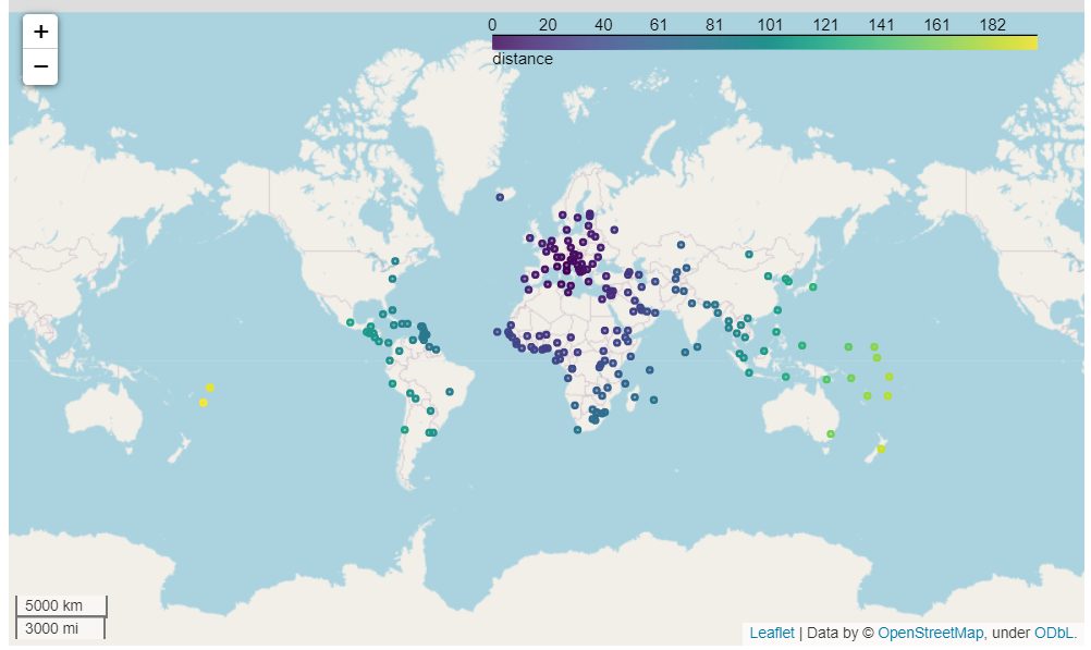
This code will get data from a GeoPanda's dataset, perform a distance calculation on the data, and then visualize it on an interactive Folium map.
Get the data
First, get the geospatial data to visualize. You can either read in a file, create a Panda's DataFrame, or create a GeoDataFrame. In this example, we will use the user input inputs['dataset'] to select a GeoPanda's and then read it in as a file.
path_to_data = geopandas.datasets.get_path(inputs['dataset'])
gdf = geopandas.read_file(path_to_data)
Manipulate the data
Once the data is loaded, we can manipulate the data using a GeoDataFrame. You can convert your data to a GeoDataFrame by passing it as the input to geopandas.GeoDataFrame(...).
In this example, we will create a new column called distance that will calculate the distance from the first point to every other point in the dataset.
In order to get a list of points, set a new column called centroid equal to the centroid of all the geometries by using the GeoPandas .centroid property.
gdf['centroid'] = gdf.centroid
Next, get the first point from the centroid column in the 0th row using .iloc[0]. Notice that iloc is a Pandas function because GeoDataFrame is an extension of Panda's DataFrame and therefore, any Pandas function can also be used on GeoDataFrame.
first_point = gdf['centroid'].iloc[0]
Now that we have a column of centroid points and the first point, we can perform the calculations. GeoPandas provides many functions for geospatial calculations. We will use the distance() function to calculate the distance of each point to the first_point.
gdf['distance'] = geopandas.GeoSeries(gdf['centroid']).distance(first_point)
Exporting the map
Finally, to export the GeoDataFrame data as an interactive Folium map, use the .explore() function and pass in "distance" as an input, where "distance" is the name of the column that you want to "explore" on the map. Then use ._repr_html_() to convert the Folium map object into an HTML string that can be displayed on the webpage.
m = gdf.explore("distance", legend=True)
interactive_map = m._repr_html_()
Step 2.2: Code version 2
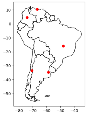
This code will create data as a Panda's DataFrame, convert it to a GeoDataFrame, and then export it as a Matplotlib plot image.
Get the data
First, create a Panda's DataFrame with the data to visualize on the map.
df = pd.DataFrame(
    {'City': ['Buenos Aires', 'Brasilia', 'Santiago', 'Bogota', 'Caracas'],
        'Country': ['Argentina', 'Brazil', 'Chile', 'Colombia', 'Venezuela'],
        'Latitude': [-34.58, -15.78, -33.45, 4.60, 10.48],
        'Longitude': [-58.66, -47.91, -70.66, -74.08, -66.86]})
Convert the DataFrame into a GeoDataFrame by passing df into geopandas.GeoDataFrame(). Then convert the latitude and longitude columns into Points using geopandas.points_from_xy(), and set these Points as the geometry column.
gdf = geopandas.GeoDataFrame(
    df, geometry=geopandas.points_from_xy(df.Longitude, df.Latitude)
)
Optionally, you can set a background for the plot. In this example, we will use a map of South America from the geopandas dataset as the background of the plot.
path_to_data = geopandas.datasets.get_path("naturalearth_lowres")
world = geopandas.read_file(path_to_data)
ax = world[world.continent == 'South America'].plot(color='white', edgecolor='black')
Exporting the map
Finally, to export the GeoDataFrame as a Matplotlib plot, use the .plot() function, and then call plt_show() to convert the Matplotlib figure into an image that can be displayed on the webpage.
m = gdf.plot(ax=ax, color="red")
static_map = plt_show(m.figure)
Step 2.3: Full Code
import geopandas
import pandas as pd
import mecsimcalc as msc


def main(inputs):
    # (i) Use a geopandas dataset
    path_to_data = geopandas.datasets.get_path(inputs['dataset'])
    gdf = geopandas.read_file(path_to_data)
    # Manipulate geospatial data
    gdf['centroid'] = gdf.centroid
    first_point = gdf['centroid'].iloc[0]
    # Calculate distance to first_point
    gdf['distance'] = geopandas.GeoSeries(
        gdf['centroid']).distance(first_point)
    mean_of_distance = gdf['distance'].mean()
    # (a) Export distance column as an interactive map
    m = gdf.explore("distance", legend=True)
    interactive_map = m._repr_html_()

    # (ii) Use a custom pandas dataset
    df = pd.DataFrame(
        {'City': ['Buenos Aires', 'Brasilia', 'Santiago', 'Bogota', 'Caracas'],
         'Country': ['Argentina', 'Brazil', 'Chile', 'Colombia', 'Venezuela'],
         'Latitude': [-34.58, -15.78, -33.45, 4.60, 10.48],
         'Longitude': [-58.66, -47.91, -70.66, -74.08, -66.86]})
    # Convert Pandas dataframe to GeoDataFrame
    gdf = geopandas.GeoDataFrame(
        # Use points_from_xy to convert to shapely.Point objects
        df, geometry=geopandas.points_from_xy(df.Longitude, df.Latitude)
    )
    # Use a map of South America
    path_to_data = geopandas.datasets.get_path("naturalearth_lowres")
    world = geopandas.read_file(path_to_data)
    ax = world[world.continent == 'South America'].plot(color='white', edgecolor='black')
    # (b) Export as a static image
    m = gdf.plot(ax=ax, color="red")
    static_map = msc.print_plot(m.figure)

    return {"interactive_map": interactive_map, "static_map": static_map, "mean_of_distance": mean_of_distance}
Step 3: Output
For the output, display the two maps: outputs.static_map and outputs.interactive_map:
{{ outputs.static_map }}

{{ outputs.interactive_map }}