Example 2: Advanced GeoPandas

This example provides a detailed explanation on how to use GeoPandas to visualize structured data.

To get started, go to mecsimcalc.com/create, click on Maps, and select Create a new blank app.

Step 1: Code

Get the data

First, import or create the geospatial data to visualize. In this example, we will create a Panda's DataFrame and then convert it into a GeoDataFrame.

Create a DataFrame with Easting and Northing coordinates.

df = pd.DataFrame({"Easting": [444246.35, 444247.044, 444247.3266, 444247.5912, 444247.8385],
                   "Northing": [5465340.18, 5465359.6118, 5465367.5256, 5465374.9338, 5465381.8589]})

df looks like this:

Easting	Northing
444246.3500	5.465340e+06
444247.0440	5.465360e+06
444247.3266	5.465368e+06
444247.5912	5.465375e+06
444247.8385	5.465382e+06

Merge the Easting and Northing columns into one column. This will make it easier to create shapes later on. The new column must be named geometry, as will be explained later.

df["geometry"] = df[["Easting", "Northing"]].values.tolist()

df looks like this:

Easting	Northing	geometry
444246.3500	5.465340e+06	[444246.35, 5465340.18]
444247.0440	5.465360e+06	[444247.044, 5465359.6118]
444247.3266	5.465368e+06	[444247.3266, 5465367.5256]
444247.5912	5.465375e+06	[444247.5912, 5465374.9338]
444247.8385	5.465382e+06	[444247.8385, 5465381.8589]

Convert the geometry column into points by applying the Point function from shapely.geometry to all the rows using .apply().

df["geometry"] = df["geometry"].apply(Point)

df looks like this:

Easting	Northing	geometry
444246.3500	5.465340e+06	POINT(444246.350 5465340.180)
444247.0440	5.465360e+06	POINT(444247.044 5465359.612)
444247.3266	5.465368e+06	POINT(444247.327 5465367.526)
444247.5912	5.465375e+06	POINT(444247.591 5465374.934)
444247.8385	5.465382e+06	POINT(444247.839 5465381.859)

Now, convert the df DataFrame into a GeoDataFrame, gdf.

gdf = geopandas.GeoDataFrame(df, crs="EPSG:26911")

Coordinate Reference System (CRS)

Notice that the coordinates are in Easting and Northing, whereas, GeoPandas expects latitude and longitude. Therefore, the coordinates must be projected into latitude and longitude. Fortunately, GeoDataFrame has a built-in crs (Coordinate Reference Systems) that applies the projection to the geometry column.

In this example, crs is "EPSG:26911", but it is likely to be different for your code, depending on which coordinate reference system is used.

tip

If your coordinates are already in latitude and longitude, then you can skip setting the crs attribute.

danger

You shapes must be in the geometry column in order for the crs projection to be applied properly!

Manipulate the data

Next, we will create more geometries in a separate GeoDataFrame, and then append it to the end of the existing GeoDataFrame, gdf.

Use LineString and Polygon to create new shapes inside a new GeoDataFrame called more_geometries.

tip

You can find more shapely geometries here.

Use pd.concat to concatenate more_geometries to the end of gdf. Note that axis=0 means to concatenate as a new row, whereas axis=1 means to concatenate as a new column.

more_geometries = geopandas.GeoDataFrame(
    {
        "geometry": [
            LineString([[444248.0694, 5.465388e06], [444248.2847, 5.465394e06], [444248.4852, 5.465400e06]]),
            Polygon([[444243.6719, 5.465405e06], [444248.8454, 5.465410e06], [444249.0068, 5.465415e06], [444299.1569, 5.465419e06]]),
        ]
    }
)
gdf = pd.concat((gdf, more_geometries), axis=0)

gdf looks like this:

Easting	Northing	geometry
444246.3500	5.465340e+06	POINT(444246.350 5465340.180)
444247.0440	5.465360e+06	POINT(444247.044 5465359.612)
444247.3266	5.465368e+06	POINT(444247.327 5465367.526)
444247.5912	5.465375e+06	POINT(444247.591 5465374.934)
444247.8385	5.465382e+06	POINT(444247.839 5465381.859)
NaN	NaN	LINESTRING(444248.069 5465388.000, 444248.285...)
NaN	NaN	POLYGON((444243.672 5465405.000, 444248.845 5...))

Now that we have defined all the geometries, we can add our computed values for each geometry as a new column called value. Here we are using some random numbers, but you should compute more meaningful numbers with the help of other libraries, such as Numpy, GeoPandas, or Pandas.

gdf["value"] = [1,2,3,4,5,6,7] # computed values

gdf looks like this:

Easting	Northing	geometry	value
444246.3500	5.465340e+06	POINT(444246.350 5465340.180)	1
444247.0440	5.465360e+06	POINT(444247.044 5465359.612)	2
444247.3266	5.465368e+06	POINT(444247.327 5465367.526)	3
444247.5912	5.465375e+06	POINT(444247.591 5465374.934)	4
444247.8385	5.465382e+06	POINT(444247.839 5465381.859)	5
NaN	NaN	LINESTRING(444248.069 5465388.000...)	6
NaN	NaN	POLYGON((444243.672 5465405.000...))	7

Exporting the map

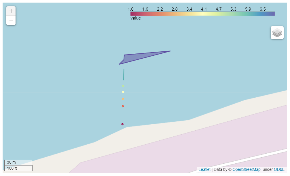
Interactive map

Export the gdf GeoDataFrame as an interactive map:

m1 = gdf.explore("value", cmap="Spectral", name="My shapes", tiles=None)
m1.options["preferCanvas"] = True

Where,

gdf.explore returns a Folium map object.
"value" is the column of gdf that contains the numerical values to be visualized.
cmap is the color of the scale. See more colormaps here.
name is the LayerControl name for the shape geometries.
tiles=None to not set a map tile. In most cases, you do not need to specify the tiles attribute.
m1.options["preferCanvas"] = True should be set to True when you are drawing lots of geometries or when the map feels slow or laggy. Otherwise, you can leave this line out.

Next, we will add a LayerControl to the map that will allow switching map tiles and toggling the geometries on and off.

Add each TileLayer separately to the map. Note that OpenStreetMap and Stamen Terrain are strings, whereas, Satellite must specify an url for tiles. This is because OpenStreetMap and Stamen Terrain are map tiles built into Folium, whereas Satellite is a custom map tile.

folium.TileLayer("OpenStreetMap", name="Road").add_to(m1)
folium.TileLayer("Stamen Terrain", name="Terrain").add_to(m1)
folium.TileLayer(
    tiles="https://server.arcgisonline.com/ArcGIS/rest/services/World_Imagery/MapServer/tile/{z}/{y}/{x}",
    attr="Esri",
    name="Satellite",
).add_to(m1)
folium.LayerControl().add_to(m1)

Finally, convert the map object to HTML that can be displayed on the webpage.

interactive_map = m1._repr_html_()

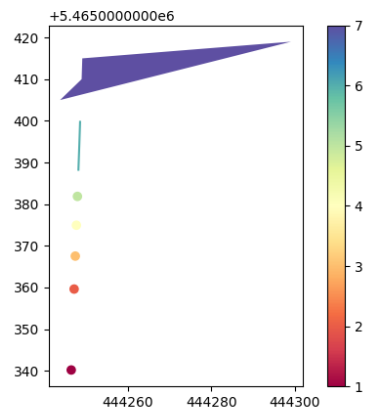
Static map

We will also export the map as a static Matplotlib plot.

import mecsimcalc as msc

m2 = gdf.plot("value", cmap="Spectral", legend=True)
static_map = msc.print_plot(m2.figure)

Where,

gdf.plot returns a Matplotlib figure.
"value" is the column of gdf that contains the numerical values to be visualized.
cmap is the color of the scale. See more colormaps here.
legend=True displays the color bar on the right.
Pass in m2.figure into plt_show to return an image that can be displayed on the webpage.

Full code

import folium
import geopandas
import pandas as pd
from shapely.geometry import LineString, Point, Polygon
import mecsimcalc as msc


def main(inputs):
    # Create data as Panda's DataFrame
    df = pd.DataFrame(
        {
            "Easting": [444246.35, 444247.044, 444247.3266, 444247.5912, 444247.8385],
            "Northing": [
                5465340.18,
                5465359.6118,
                5465367.5256,
                5465374.9338,
                5465381.8589,
            ],
        }
    )
    # Merge `Easting` and `Northing` columns into one column called `geometry`
    df["geometry"] = df[["Easting", "Northing"]].values.tolist()
    # Convert all geometries into Point shapes
    df["geometry"] = df["geometry"].apply(Point)

    # Convert DataFrame to GeoDataFrame and project coordinates to "EPSG:26911"
    gdf = geopandas.GeoDataFrame(df, crs="EPSG:26911")

    # Create a new GeoDataFrame with a LineString and a Polygon
    more_geometries = geopandas.GeoDataFrame(
        {
            "geometry": [
                LineString(
                    [
                        [444248.0694, 5.465388e06],
                        [444248.2847, 5.465394e06],
                        [444248.4852, 5.465400e06],
                    ]
                ),
                Polygon(
                    [
                        [444243.6719, 5.465405e06],
                        [444248.8454, 5.465410e06],
                        [444249.0068, 5.465415e06],
                        [444299.1569, 5.465419e06],
                    ]
                ),
            ]
        }
    )
    # Add the new geometries as new rows to the existing GeoDataFrame, gdf
    gdf = pd.concat((gdf, more_geometries), axis=0)

    # Add computed values as a new column to gdf
    gdf["value"] = [1, 2, 3, 4, 5, 6, 7]  # computed values

    # Export gdf as an interactive Folium map
    m1 = gdf.explore("value", cmap="Spectral", name="My shapes", tiles=None)
    # Set `preferCanvas` to optimize performance of map
    m1.options["preferCanvas"] = True

    # Add a LayerControl with different TileLayers
    folium.TileLayer("OpenStreetMap", name="Road").add_to(m1)
    folium.TileLayer("Stamen Terrain", name="Terrain").add_to(m1)
    folium.TileLayer(
        tiles="https://server.arcgisonline.com/ArcGIS/rest/services/World_Imagery/MapServer/tile/{z}/{y}/{x}",
        attr="Esri",
        name="Satellite",
    ).add_to(m1)
    folium.LayerControl().add_to(m1)

    # Get Folium map as HTML string
    interactive_map = m1._repr_html_()

    # Export gdf as Matplotlib plot image
    m2 = gdf.plot("value", cmap="Spectral", legend=True)
    static_map = msc.print_plot(m2.figure)

    return {"interactive_map": interactive_map, "static_map": static_map}

Step 2: Output

{{ outputs.interactive_map }}
{{ outputs.static_map }}

Step 1: Code​

Get the data​

Coordinate Reference System (CRS)​

Manipulate the data​

Exporting the map​

Interactive map​

Static map​

Full code​

Step 2: Output​

Step 1: Code

Get the data

Coordinate Reference System (CRS)

Manipulate the data

Exporting the map

Interactive map

Static map

Full code

Step 2: Output